Chapter 3 Technical Matters

3.1 The Generalised Rasch Model

The model fitted by ACER ConQuest is a generalised multidimensional Rasch item response model coupled with a multivariate regression model. We call these two components of the model the item response model and the population model respectively. As we have illustrated in previous sections, the model allows ACER ConQuest to be used for two important types of analyses.

First, the general specification of the item response model allows us to use one model to fit a wide variety of Rasch models. In the unidimensional case, this includes the simple logistic model (Wright & Panchapakesan, 1969), the linear logistic model (Fischer, 1973), the rating scale and partial credit models (Andrich, 1978; Glas, 1989; Masters, 1982), the ordered partition model (Wilson, 1992), and multifaceted models (Linacre, 1994). Furthermore, multidimensional dichotomous and polytomous response models, such as Kelderman’s LOGIMO model (Kelderman & Rijkes, 1994), Rasch’s multidimensional model (Rasch, 1980), and the models of Whitely (1980), Andersen (1985) and Embretson (1991), can also be shown to be special cases of the generalised multidimensional Rasch model.

Second, the combination of the item response and population models allows ACER ConQuest to be used to undertake latent regression. The term latent regression refers to the direct estimation of regression models from item response data. To illustrate the use of latent regression, consider the following typical situation. We have two groups of students, group A and group B, and we are interested in estimating the difference in the mean achievement of the two groups. If we follow standard practice, we will administer a common test to the students and then use this test to produce achievement scores for all of the students. We could then follow a standard procedure, such as regression (which, in this simple case, becomes identical to a t-test), to examine the difference in the means. Depending upon the method that is used to construct the achievement scores, this approach can result in misleading inferences about the differences in the means. Using the latent regression methods described by Adams, Wilson, & Wu (1997), ACER ConQuest avoids such problems by directly estimating the difference in the achievement of the groups from the response data.

3.1.1 The Item Response Model

The item response model fitted by ACER ConQuest is the multidimensional random coefficients multinomial logit model that was described by Adams, Wilson, & Wang (1997). For ease of explanation, we will first describe the unidimensional form of the model.

3.1.1.1 The Unidimensional Random Coefficients Multinomial Logit Model

Assume that \(I\) items are indexed \(i = 1, ..., I\), with each item admitting \(K_i + 1\) response alternatives \(k=0,1,...,K_i\). Use the vector-valued random variable \(X'_i = (X_{i1}, X_{i2}, ..., X_{iK_i})\), where

\[\begin{equation} X_{ij}=\left\{\begin{array}{cc} 1 & \mbox{if the response to item i is in category j}\\0 & \mbox{otherwise}\end{array}\right. \text{,} \tag{3.1} \end{equation}\]

to indicate the \(K_i + 1\) possible responses to item \(i\).

A response in category zero is denoted by a vector of zeroes. This effectively makes the zero category a reference category and is necessary for model identification. The choice of this as the reference category is arbitrary and does not affect the generality of the model. We can also collect the \(X_i\) together into the single vector \(X' = (X'_1, X'_2, ..., X'_l)\), which we call the response vector (or pattern). Particular instances of each of these random variables are indicated by their lower case equivalents: \(x\), \(x_i\) and \(x_{ik}\).

The items are modelled through a vector \(\xi' = (\xi_1, \xi_2, ..., \xi_p)\) of \(P\)parameters. Linear combinations of these are used in the response probability model to describe the empirical characteristics of the response categories of each item. These linear combinations are defined by design vectors \(a_{ik'}(i=1, ..., I;k=1, ..., K_i)\), each of length \(P\), which can be collected to form a design matrix \(A' = (a_{11}, a_{12}, ..., a_{1K_1}, a_{21}, a_{22}, ..., a_{2K_2}, ..., a_{I1}, ..., a_{IK_I})\). Adopting a very general approach to the definition of items, in conjunction with the imposition of a linear model on the item parameters, allows us to write a general model that includes the wide class of existing Rasch models mentioned above and to develop new types of Rasch models (for example, the item bundles models of Wilson & Adams (1995)).

An additional feature of the model is the introduction of a scoring function that allows the specification of the score or ‘performance level’ that is assigned to each possible response to each item. To do this, we introduce the notion of a response score \(b_{ij}\), which gives the performance level of an observed response in category \(j\) of item \(i\). The \(b_{ij}\) can be collected in a vector as \(b' = (b_{11}, b_{12}, ..., b_{1K_1}, b_{21}, b_{22}, ..., b_{2K_2}, ..., b_{I1}, ..., b_{IK_I})\). (By definition, the score for a response in the zero category is zero, but other responses may also be scored zero.)

In the majority of Rasch model formulations, there has been a one-to-one match between the category to which a response belongs and the score that is allocated to the response. In the simple logistic model, for example, it has been standard practice to use the labels \(0\) and \(1\) to indicate both the categories of performance and the scores. A similar practice has been followed with the rating scale and partial credit models, where each different possible response is seen as indicating a different level of performance, so that the category indicators \(0\), \(1\), \(2\) etc. that are used serve both as scores and labels. The use of \(b\) as a scoring function allows a more flexible relationship between the qualitative aspects of a response and the level of performance that it reflects. Examples of where this is applicable are given in Kelderman & Rijkes (1994) and Wilson (1992).

Letting \(\theta\) be the latent variable, the item response probability model is written as

\[\begin{equation} Pr(X_{ij}=1;A,b,\xi|\theta) = \frac{exp(b_{ij}\theta+a'_{ij}\xi)}{\sum^{K_i}_{k=1}exp(b_{ik}\theta+a'_{ij}\xi)} \text{,} \tag{3.2} \end{equation}\]

and a response vector probability model as

\[\begin{equation} f(x;\xi|\theta)=\Psi(\theta, \xi)exp[x'(b\theta+A\xi)] \text{,} \tag{3.3} \end{equation}\]

with \[\begin{equation} \Psi(\theta, \xi) = \{\sum_{z\in\Omega}exp[z'(b\theta+A\xi)]\}^{-1} \text{,} \tag{3.4} \end{equation}\]

where \(\Omega\) is the set of all possible response vectors.

3.1.1.2 The Multidimensional Random Coefficients Multinomial Logit Model

The multidimensional form of the model is a straightforward extension of the unidimensional model. It assumes that a set of \(D\) latent traits underlies the individuals’ responses. The \(D\) latent traits define a \(D\)-dimensional latent space, and the individuals’ positions in the \(D\)-dimensional latent space are represented by the vector \(\theta = (\theta_1, \theta_2, ..., \theta_D)\). The scoring function of response category \(k\) in item \(i\) now corresponds to a \(D\)-by-\(1\)-column vector rather than to a scalar as in the unidimensional model. A response in category \(k\) in dimension \(d\) of item \(i\) is scored \(b_{ikd}\). The scores across \(D\) dimensions can be collected into a column vector \(b'_{ik} = (b_{ik1}, b_{ik2}, ..., b_{ikD})\) then collected into the scoring submatrix for item \(i\), \(B'_i = (b_{i1}, b_{i2}, ..., b_{iK_i})\) and then collected into a scoring matrix \(B'=(B'_1, B'_2, ..., B'_I)\) for the whole test. If the item parameter vector, \(p\), and the design matrix, \(A\), are defined as they were in the unidimensional model, the probability of a response in category \(k\) of item \(i\) is modelled as

\[\begin{equation} Pr(X_{ij}=1;A,B,\xi|\theta) = \frac{exp(b'_{ij}\theta+a'_{ij}\xi)}{\sum^{K_i}_{k=1}exp(b'_{ik}\theta+a'_{ik}\xi)} \text{.} \tag{3.5} \end{equation}\]

And for a response vector we have

\[\begin{equation} f(x;\xi|\theta)=\Psi(\theta, \xi)exp[x'(B\theta+A\xi)] \text{,} \tag{3.6} \end{equation}\]

with \[\begin{equation} \Psi(\theta, \xi) = \left\{\sum_{z\in\Omega}exp[z'(B\theta+A\xi)]\right\}^{-1} \text{.} \tag{3.7} \end{equation}\]

The difference between the unidimensional model and the multidimensional model is that the ability parameter is a scalar, \(\theta\), in the former, and a \(D\)-by-\(1\)-column vector, \(b_{ik}\), in the latter. Likewise, the scoring function of response \(k\) to item \(i\) is a scalar, \(b_{ik}\), in the former, whereas it is a \(D\)-by-\(1\)-column vector, \(b_{ik}\), in the latter.

For the purposes of the identification of (3.6), certain constraints must be placed on the design matrices A and B. Volodin & Adams (1995) show that the following are necessary and sufficient conditions for the identification of (3.6).

• Proposition One:
  If \(D\) is the number of latent dimensions, \(P\) is the length of the parameter vector, \(\xi\), \(K_i + 1\) is the number of response categories for item \(i\), and \(K = \sum_{i\in I} K_i\), then model (3.6) if applied to the set of items \(I\) can only be identified if \(P+D \leq K\).

• Proposition Two:
  If \(D\) is the number of latent dimensions and \(P\) is the length of the parameter vector, \(\xi\), then model (3.6) can only be identified if \(rank(A) = P\), \(rank(B) = D\) and \(rank(BA)= P + D\).

• Proposition Two:
  If \(D\) is the number of latent dimensions, \(P\) is the length of the parameter vector, \(\xi\), \(K_1 + 1\) is the number of response categories for item \(i\), and \(K=\sum_{i\in 1}K_i\), then model (3.6) if applied to the set of items \(I\) can only be identified if and only if \(rank([BA]) = P + D \leq K\).

3.1.2 The Population Model

The item response model is a conditional model, in the sense that it describes the process of generating item responses conditional on the latent variable, \(\theta\). The complete definition of the model, therefore, requires the specification of a density, \(f_\theta(\theta;\alpha)\), for the latent variable, \(\theta\). We use \(\alpha\) to symbolise a set of parameters that characterise the distribution of \(\theta\). The most common practice when specifying unidimensional marginal item response models is to assume that the students have been sampled from a normal population with mean \(\mu\) and variance \(\sigma^2\). That is:

\[\begin{equation} f_\theta(\theta;\alpha) \equiv f_\theta(\theta;\mu,\sigma^2) = \frac{1}{\sqrt{2\pi\sigma^2}}exp\left[-\frac{(\theta-\mu)^2}{2\sigma^2}\right] \tag{3.8} \end{equation}\]

or equivalently

\[\begin{equation} \theta = \mu + E \tag{3.9} \end{equation}\]

where \(E \sim N(0, \sigma^2).\)

Adams, Wilson, & Wu (1997) discuss how a natural extension of (3.8) is to replace the mean, \(n\), with the regression model \(Y'_n\beta\), where \(Y_n\) is a vector of \(u\) fixed and known values for student \(n\) and \(\beta\) is the corresponding vector of regression coefficients. For example, \(Y_n\) could be constituted of student variables, such as gender, socio-economic status, or major. Then the population model for student \(n\) becomes

\[\begin{equation} \theta_n = Y'_n\beta + E_{n\prime} \text{,} \tag{3.10} \end{equation}\]

where we assume that the \(E_n\) are independently and identically normally distributed with mean zero and variance \(\sigma^2\) so that (3.10) is equivalent to

\[\begin{equation} f_\theta(\theta_n; Y_n, \beta, \sigma^2) = (2\pi\sigma^2)^{-\frac12}exp\left[-\frac1{2\sigma^2}(\theta_n-Y'_n\beta)'(\theta_n-Y'_n\beta)\right] \text{,} \tag{3.11} \end{equation}\]

a normal distribution with mean \(Y'_n\beta\) and variance \(\sigma^2\). If (3.11) is used as the population model, then the parameters to be estimated are \(\beta\), \(\sigma^2\) and \(\xi\).

The model takes the generalisation one step further by applying it to the vector-valued \(\theta\) rather than the scalar-valued \(\theta\), resulting in the multivariate population model

\[\begin{equation} f_\theta(\theta_n;W_n,\gamma,\Sigma) = (2\pi)^{-\frac d2}|\Sigma|^{-\frac12}exp\left[-\frac12(\theta_n-\gamma W_n)' \Sigma^{-1}(\theta_n - \gamma W_n)\right] \text{,} \tag{3.12} \end{equation}\]

where \(\gamma\) is a \(u\)-by-\(d\) matrix of regression coefficients, \(\Sigma\) is a \(d\)-by-\(d\) variance-covariance matrix and \(W_n\) is a \(u\)-by-\(1\) vector of fixed variables. If (3.12) is used as the population model, then the parameters to be estimated are \(\gamma\), \(\Sigma\) and \(\xi\).

3.1.3 Estimation

ACER ConQuest uses maximum likelihood methods to provide estimates of c, R and p. Combining the conditional item response model (3.6) and the population model (3.12), we obtain the unconditional, or marginal, item response model

\[\begin{equation} f_x(x; \xi, \gamma, \Sigma) = \int_\theta f_x (x; \xi| \theta)f_\theta(\theta; \gamma, \Sigma)d\theta \text{,} \tag{3.13} \end{equation}\]

and it follows that the likelihood is

\[\begin{equation} \Lambda = \prod^N_{n=1} f_x(x_n; \xi, \gamma, \Sigma) \text{,} \tag{3.14} \end{equation}\]

where \(N\) is the total number of sampled students.

Differentiating with respect to each of the parameters and defining the marginal posterior as

\[\begin{equation} h_\theta(\theta_n;W_n,\xi,\gamma,\Sigma|x_n) = \frac{f_x(x_n;\xi|\theta_n)f_\theta(\theta_n;W_n,\gamma,\Sigma)}{f_x(x_n;W_n,\xi,\gamma,\Sigma)} \tag{3.15} \end{equation}\] provides the following system of likelihood equations:

\[\begin{equation} A' \sum_{n=1}^N\left[x_n-\int_{\theta_n}E_z(z|\theta_n)h_\theta(\theta_n;Y_n,\xi,\gamma,\Sigma|x_n)d\theta_n\right]=0 \text{,} \tag{3.16} \end{equation}\]

\[\begin{equation} \hat{\gamma} = \left(\sum_{n=1}^N\bar{\theta_n}W'_n\right)\left(\sum_{n=1}^NW_nW'_n\right)^{-1} \text{,} \tag{3.17} \end{equation}\] \[\begin{equation} \hat{\Sigma}=\frac1N\sum_{n=1}^N\int_{\theta_n}(\theta_n-\gamma W_n)(\theta_n-\gamma W_n)'h_\theta(\theta_n;Y_n,\xi,\gamma,\Sigma|x_n)d\theta_n \text{,} \tag{3.18} \end{equation}\]

where

\[\begin{equation} E_{z}\left(z | \theta_{n}\right)=\Psi\left(\theta_{n}, \xi\right) \sum_{z \in \Omega} z \exp \left[z^{\prime}\left(b \theta_{n}+A \xi\right)\right] \text{;} \tag{3.19} \end{equation}\]

and

\[\begin{equation} \overline{\theta}_{n}=\int_{\theta_{n}} \theta_{n} h_{\theta}\left(\theta_{n} ; Y_{n}, \xi, \gamma, \Sigma | x_{n}\right) d \theta_{n} \text{.} \tag{3.20} \end{equation}\]

The system of equations defined by (3.16), (3.17) and (3.18) is solved using an EM algorithm (Dempster et al., 1977) following the approach of Bock & Aitkin (1981).

3.1.3.1 Quadrature and Monte Carlo Approximations

The integrals in equations (3.16), (3.17) and (3.18) are approximated numerically using either quadrature or Monte Carlo methods. In each case, we define \(\Theta_q\) and a set of \(Q\) \(D\)-dimensional vectors (which we call nodes); and for each node we define a corresponding weight \(W_q(\gamma, \Sigma)\). The marginal item response probability (3.13) is then approximated using

\[\begin{equation} f_{x}(x ; \xi, \gamma, \Sigma) \approx \sum_{p=1}^{Q} f_{x}\left(x ; \xi | \Theta_{p}\right) W_{p}(\gamma, \Sigma) \text{;} \tag{3.21} \end{equation}\]

and the marginal posterior (3.15) is approximated using

\[\begin{equation} h_{\Theta}\left(\Theta_{q} ; W_{n}, \xi, \gamma, \Sigma | x_{n}\right) \approx \frac{f_{x}\left(x_{n} ; \xi | \Theta_{q}\right) W_{q}(\gamma, \Sigma)}{\sum_{p=1}^{Q} f_{x}\left(x_{n} ; \xi | \Theta_{p}\right) W_{p}(\gamma, \Sigma)} \tag{3.22} \end{equation}\]

for \(q = 1, ..., Q\).

The EM algorithm then proceeds as follows:

1. Prepare a set of nodes and weights depending upon \(\gamma^{(t)}\) and \(\Sigma^{(t)}\) which are the estimates of \(\gamma\) and \(\Sigma\) at iteration \(t\).

2. Calculate the discrete approximation of the marginal posterior density of \(\Theta_n\), given \(x_n\) at iteration \(t\), using

   \[\begin{equation} h_{\Theta}\left(\Theta_{q} ; W_{n}, \xi^{(t)}, \boldsymbol{\gamma}^{(t)}, \boldsymbol{\Sigma}^{(t)} | x_{n}\right)= \frac{f_{x}\left(x_{n} ; \xi^{(t)} | \boldsymbol{\Theta}_{q}\right) W_{q}\left(\gamma^{(t)}, \Sigma^{(t)}\right)}{\sum_{p=1}^{Q} f_{x}\left(x_{n} ; \xi^{(t)} | \boldsymbol{\Theta}_{p}\right) W_{p}\left(\gamma^{(t)}, \Sigma^{(t)}\right)} \text{,} \tag{3.23} \end{equation}\]

   where \(\xi^{(t)}\), \(\gamma^{(t)}\) and \(\Sigma^{(t)}\) are estimates of \(\xi\), \(\gamma\) and \(\Sigma\) at iteration \(t\).

3. Use the Newton-Raphson method to solve the following to produce estimates of \(\xi^{(t+1)}\)

   \[\begin{equation} A^{\prime} \sum_{n=1}^{N}\left[x_{n}-\sum_{r=1}^{Q} E_{z}\left(z | \Theta_{r}\right) h_{\Theta}\left(\Theta_{r} ; W_{n}, \xi^{(t)}, \boldsymbol{\gamma}^{(t)}, \boldsymbol{\Sigma}^{(t)} | x_{n}\right)\right] = 0 \text{.} \tag{3.24} \end{equation}\]

4. Estimate \(\gamma^{(t+1)}\) and \(\Sigma^{(t+1)}\), using

   \[\begin{equation} \gamma^{(t+1)} = \left(\sum_{n=1}^{N} \overline{Q}_{n} W_{n}^{\prime}\right)\left(\sum_{n=1}^{N} W_{n} W_{n}^{\prime}\right)^{-1} \tag{3.25} \end{equation}\] and \[\begin{equation} \begin{split} \Sigma^{(t+1)} = \frac{1}{N} \sum_{n=1}^{N} \sum_{r=1}^{Q} & \left(\Theta_{r} -\gamma^{(t+1)} W_{n}\right)\left(\Theta_{r}-\gamma^{(t+1)} W_{n}\right)^{\prime} \\ & \cdot h_{\Theta}\left(\Theta_{r} ; Y_{n}, \xi^{(t)}, \gamma^{(t)}, \Sigma^{(t)} | x_{n}\right) \text{,} \end{split} \tag{3.26} \end{equation}\]

   where

   \[\begin{equation} \overline{\Theta}_{n}=\sum_{r=1}^{Q} \Theta_{r} h_{\Theta}\left(\Theta_{r} ; W_{n}, \xi^{(t)}, \gamma^{(t)}, \Sigma^{(t)} | x_{n}\right) \text{.} \tag{3.27} \end{equation}\]

5. Return to step 1.

The difference between the quadrature and Monte Carlo methods lies in the way the nodes and weights are prepared. For the quadrature case, we begin by choosing a fixed set of \(Q\) points, (\(\Theta_{d1}, \Theta_{d2}, ..., \Theta_{dQ}\)), for each latent dimension \(d\) and then define a set of \(Q^D\) nodes that are indexed \(r = 1, ..., Q^D\) and are given by the Cartesian coordinates

\[\begin{gather*} \Theta_{r}=\left(\Theta_{1 j_{1}}, \Theta_{2 j_{2}}, \ldots, \Theta_{D j_{D}}\right) \\ \text{with} \quad j_1=1,\ldots,Q; \quad j_2=1,\ldots,Q; \quad j_D = 1,\ldots,Q \text{.} \end{gather*}\]

The weights are then chosen to approximate the continuous multivariate latent population density (3.12). That is,

\[\begin{equation} W_{r}=K(2 \pi)^{-\frac{d}{2}}|\Sigma|^{-\frac{1}{2}} \exp \left[-\frac{1}{2}\left(\boldsymbol{\Theta}_{r}-\boldsymbol{\gamma} W_{n}\right)^{\prime} \boldsymbol{\Sigma}^{-1}\left(\boldsymbol{\Theta}_{r}-\boldsymbol{\gamma} W_{n}\right)\right] \text{,} \tag{3.28} \end{equation}\]

where \(K\) is a scaling factor to ensure that the sum of the weights is \(1\).

In the Monte Carlo case, the nodes are drawn at random from the standard multivariate normal distribution; and at each iteration, the nodes are rotated, using standard methods, so that they become random draws from a multivariate normal distribution with mean \(\gamma W_n\) and variance \(\Sigma\). In the Monte Carlo case, the weight for all nodes is \(1/Q\).

For further information on the quadrature approach to estimating the model, see Adams, Wilson, & Wang (1997); and for further information on the Monte Carlo estimation method, see Volodin & Adams (1995).

3.1.3.2 Estimating Standard Errors

Asymptotic standard errors for the parameter estimates are estimated using the observed Fisher’s information. For the unidimensional case, a derivation of the formulae for the observed information is provided in Adams, Wilson, & Wu (1997).³⁷

If the observed information matrix is written as

\[\begin{equation} I=\left[\begin{array}{ccc} {I_{\xi \xi^{\prime}}} & {I_{\beta \xi^{\prime}}} & {I_{\sigma^{2} \xi^{\prime}}} \\ {I_{\xi \beta^{\prime}}} & {I_{\beta \beta^{\prime}}} & {I_{\sigma^{2} \beta^{\prime}}} \\ {I_{\xi \sigma^{2}}} & {I_{\beta \sigma^{2}}} & {I_{\left(\sigma^{2}\right)^{2}}} \end{array}\right] \text{,} \tag{3.29} \end{equation}\]

Adams, Wilson, & Wu (1997) show that, for the unidimensional model, the components of the matrix are

\[\begin{equation} \begin{split} I_{\xi \xi'} = & -A^{\prime} \sum_{n=1}^{N}\left[\int_{\theta_{n}} E_{z}\left(z z^{\prime} | \theta_{n}\right) h_{\theta}\left(\theta_{n} ; Y_{n}, \hat{\xi}, \hat{\beta}, \hat{\sigma}^{2} | x_{n}\right) d \theta_{n} \right. \\ & -2 \int_{\theta_{n}} E_{z}\left(z | \theta_{n}\right) E_{z}\left(z^{\prime} | \theta_{n}\right) h_{\theta}\left(\theta_{n} ; Y_{n}, \hat{\xi}, \hat{\beta}, \hat{\sigma}^{2} | x_{n}\right) d \theta_{n} \\ & +\int_{\theta_{n}} E_{z}\left(z | \theta_{n}\right) h_{\theta}\left(\theta_{n} ; Y_{n}, \hat{\xi}, \hat{\beta}, \hat{\sigma}^{2} | x_{n}\right) d \theta_{n} \\ & \left. \qquad \cdot \int_{\theta_{n}} E_{z}\left(z^{\prime} | \theta_{n}\right) h_{\theta}\left(\theta_{n} ; Y_{n}, \hat{\xi}, \hat{\beta}, \hat{\sigma}^{2} | x_{n}\right) d \theta_{n} \right] A \text{,} \end{split} \tag{3.30} \end{equation}\]

\[\begin{equation} I_{\beta \beta^{\prime}}=\sum_{n=1}^{N} \frac{Y_{n} Y_{n}^{\prime}}{\hat{\sigma}^{2}}\left[\frac{\hat{E}_{\theta}\left(\theta_{n}^{2}\right)-\hat{E}_{\theta}\left(\theta_{n}\right)^{2}}{\hat{\sigma}^{2}}-1\right] \text{,} \tag{3.31} \end{equation}\]

\[\begin{equation} \begin{split} I_{\left(\sigma^{2}\right)^{2}}= -\frac{N}{2 \hat{\sigma}^{4}}+ \frac{1}{4 \hat{\sigma}^{8}} \sum_{n=1}^{N} & \left[\int_{\theta_{n}}\left(\theta_{n}-Y_{n}^{\prime} \hat{\boldsymbol{\beta}}\right)^{4} h_{\theta}\left(\theta_{n} ; Y_{n^{\prime}}, \hat{\boldsymbol{\xi}}, \hat{\beta}, \hat{\sigma}^{2} | x_{n}\right) d \theta_{n} \right. \\ & \left. -\left(\int_{\theta_{n}}\left(\theta_{n}-Y_{n}^{\prime} \hat{\boldsymbol{\beta}}\right)^{2} h_{\theta}\left(\theta_{n} ; Y_{n}, \hat{\xi}, \hat{\beta}, \hat{\sigma}^{2} | x_{n}\right) d \theta_{n}\right)^{2} \right] \text{,} \end{split} \tag{3.32} \end{equation}\]

\[\begin{equation} \begin{split} I_{\beta \xi'}=-A^{\prime} \sum_{n=1}^{N} & \left(\int_{\theta_{n}} \theta_{n} \hat{E}_{z}\left(z | \theta_{n}\right) h_{\theta}\left(\theta_{n} ; Y_{n}, \hat{\xi}, \hat{\boldsymbol{\beta}}, \hat{\sigma}^{2} | x_{n}\right) d \theta_{n}\right. \\ & \left. -\hat{E}_{\theta}\left[\hat{E}_{z}\left(z | \theta_{n}\right) \hat{E}_{\theta}\left(\theta_{n}\right)\right]\Biggr) \frac{Y_{n}^{\prime}}{\hat{\sigma}^{2}} \text{,} \right. \end{split} \tag{3.33} \end{equation}\]

\[\begin{equation} \begin{split} I_{\sigma^{2} \beta^{\prime}}=-\frac{A^{\prime}}{2 \sigma^{4}} \sum_{n=1}^{N} & \left[\int_{\theta_{n}} \hat{E}_{z}\left(z | \theta_{n}\right)\left(\theta_{n}-Y_{n}^{\prime} \hat{\boldsymbol{\beta}}\right)^{2} h_{\theta}\left(\theta_{n} ; Y_{n}, \hat{\xi}, \hat{\beta}, \hat{\sigma}^{2} | x_{n}\right) d \theta_{n} \right. \\ & -\int_{\theta_{n}} \hat{E}_{z}\left(z | \theta_{n}\right) h_{\theta}\left(\theta_{n} ; Y_{n}, \hat{\xi}, \hat{\beta}, \hat{\sigma}^{2} | x_{n}\right) d \theta_{n} \\ & \left. \qquad \cdot \int_{\theta_{n}}\left(\theta_{n}-Y_{n}^{\prime} \hat{\boldsymbol{\beta}}\right)^{2} h_{\theta}\left(\theta_{n} ; Y_{n}, \hat{\xi}, \hat{\beta}, \hat{\sigma}^{2} | x_{n}\right) d \theta_{n} \right] \text{,} \end{split} \tag{3.34} \end{equation}\]

\[\begin{equation} \begin{split} I_{\sigma^{2} \xi^{\prime}}=-\frac{1}{2 \hat{\sigma}^{6}} \sum_{n=1}^{N} & \left[\int_{\theta_{n}} Y_{n}\left(\theta_{n}-Y_{n}^{\prime} \hat{\boldsymbol{\beta}}\right)^{3} h_{\theta}\left(\theta_{n} ; Y_{n}, \hat{\xi}, \hat{\beta}, \hat{\sigma}^{2} | x_{n}\right) d \theta_{n} \right. \\ & -\int_{\theta_{n}} Y_{n}\left(\theta_{n}-Y_{n}^{\prime} \hat{\boldsymbol{\beta}}\right) h_{\theta}\left(\theta_{n} ; Y_{n}, \hat{\xi}, \hat{\boldsymbol{\beta}}, \hat{\sigma}^{2} | x_{n}\right) d \theta_{n} \\ & \left. \qquad \cdot \int_{\theta_{n}}\left(\theta_{n}-Y_{n}^{\prime} \hat{\boldsymbol{\beta}}\right)^{2} h_{\theta}\left(\theta_{n} ; Y_{n}, \hat{\xi}, \hat{\boldsymbol{\beta}}, \hat{\sigma}^{2} | x_{n}\right) d \theta_{n} \right] \text{.} \end{split} \tag{3.35} \end{equation}\]

The estimation of asymptotic standard errors using the observed information can be very time-consuming. The matrix that is computed is of dimension \(p + r + 2\) where \(p\) is the number of item parameters and \(r\) is the number of regression variables; and the computation of each element requires integration over the posterior distribution of each case. The time taken is therefore quadratic in the number of parameters and linear in the number of cases and nodes. Because the estimation of these errors can take considerable time (and memory), ACER ConQuest provides an option to compute quick approximations for the error variances, given by:

\[\begin{equation} \begin{split} \operatorname{var}\left(\hat{\xi}_{i}\right)=\sum_{n=1}^{N} & \left\{\operatorname{diag}\left[A^{\prime}\left(\int_{\theta_{n}} E_{z}\left(z z^{\prime} | \theta_{n}\right) h_{\theta}\left(\theta_{n} ; Y_{n}, \hat{\xi}, \hat{\beta}, \hat{\sigma}^{2} | x_{n}\right) d \theta_{n} \right. \right. \right. \\ & \left. \left. \left. \qquad -\int_{\theta_{n}} E_{z}\left(z | \theta_{n}\right) E_{z}\left(z^{\prime} | \theta_{n}\right) h_{\theta}\left(\theta_{n} ; Y_{n}, \hat{\xi}, \hat{\beta}, \hat{\sigma}^{2} | x_{n}\right) d \theta_{n} \right) A \right] \right\}^{-1} \end{split} \tag{3.36} \end{equation}\]

\[\begin{equation} \operatorname{var}\left(\hat{\boldsymbol{\beta}}_{i}\right)=\hat{\sigma}^{2}\left(\sum_{n=1}^{N} Y_{n} Y_{n}^{T}\right)^{-1} \tag{3.37} \end{equation}\]

\[\begin{equation} \operatorname{var}\left(\hat{\sigma}^{2}\right) = \frac{2 \hat\sigma^{4}}{N} \tag{3.38} \end{equation}\]

These approximations ignore all of the covariances in the parameter estimates. The approximations of the item parameters (3.36) will generally underestimate the sampling error, particularly for parameters associated with facets that have few levels for the step parameters in multicategory items. The accuracy of (3.37) and (3.38) depends upon the magnitude of the measurement error as it is reflected in the variances of the individual’s posterior distributions.

To choose the estimation procedure for standard errors, see the estimate command (in the Command Reference), particularly the option stderr, which can be set to use the full observed information matrix (3.29) or equations (3.36) through (3.38).

3.1.3.3 Latent Estimation and Prediction

The marginal item response model (3.13) does not include parameters for the latent values \(\theta_n\); and hence, the estimation algorithm does not result in estimates of the latent values. ACER ConQuest provides expected a-posteriori (EAP) ability estimates and maximum likelihood ability estimates of the latent quantities. The EAP ability estimate³⁸ of the latent quantity for case \(n\) is

\[\begin{equation} \theta_{n}^{E A P}=\sum_{r=1}^{Q} \Theta_{r} h_{\Theta}\left(\Theta_{r} ; W_{n}, \hat{\xi}, \hat{\gamma}, \hat{\Sigma} | \mathrm{x}_{n}\right) \text{.} \tag{3.39} \end{equation}\]

Variance estimates for these predictions are estimated using

\[\begin{equation} \operatorname{var}\left(\theta_{n}^{E A P}\right)=\sum_{r=1}^{Q}\left(\Theta_{r}-\theta_{n}^{E A P}\right)\left(\Theta_{r}-\theta_{n}^{E A P}\right)^{\prime} h_{\Theta}\left(\Theta_{r} ; W_{n}, \hat{\xi}, \hat{\gamma}, \hat{\Sigma} | x_{n}\right) \text{.} \tag{3.40} \end{equation}\]

Maximum likelihood ability estimates of the latent quantities are produced by maximising (3.6) with respect to \(\theta_n\), that is, solving the likelihood equations

\[\begin{equation} \sum_{i \in \Omega}\left[b_{i x_{n i}}-\sum_{j=1}^{K_{i}} \frac{b_{i j} \exp \left(b_{i j} \theta_{n}+a_{i j}^{\prime} \hat{\xi}\right)}{\sum_{k=1}^{K_i} \exp \left(b_{i k} \theta_{n}+a_{i k}^{\prime} \hat{\xi}\right)}\right]=0 \tag{3.41} \end{equation}\]

for each case, where \(\hat\xi\) is the vector of item parameter estimates. These equations are solved using a routine based on the Newton-Raphson method. Solving (3.41) will not produce finite estimates for cases that have responded in the lowest scoring category of each item or for cases that have responded in the highest scoring category of each item. To provide finite estimates for such cases, we add a small constant value to the scores of those cases who have responded in the lowest category, and we subtract a small constant from the scores of those cases who have responded in the highest category.³⁹

3.1.3.4 Drawing Plausible Values

Plausible values are random draws from the marginal posterior (3.15) for each student. For details on the uses of plausible values, the reader is referred to Mislevy (1991) and Mislevy et al. (1992). Unlike previously described methods for drawing plausible values (Beaton, 1987; Mislevy et al., 1992), ACER ConQuest does not assume normality of the marginal posterior distributions. Recall from (3.15) that the marginal posterior is given by

\[\begin{equation} h_\theta(\theta_n;W_n,\xi,\gamma,\Sigma|x_n) = \frac{f_x(x_n;\xi|\theta_n)f_\theta(\theta_n;W_n,\gamma,\Sigma)}{\int_\theta f_x(x; \xi | \theta) f_\theta(\theta, \gamma, \Sigma) d\theta} \text{.} \tag{3.42} \end{equation}\]

The ACER ConQuest procedure begins drawing \(M\) vector-valued random deviates, \(\left\{\varphi_{m n}\right\}_{m=1}^{M}\) from the multivariate normal distribution, \(f_\theta(\theta_n; W_n, \gamma, \Sigma)\), for each case \(n\).⁴⁰ These vectors are used to approximate the integral in the denominator of (3.42), using the Monte Carlo integration

\[\begin{equation} \int_{\theta} f_{x}(x ; \xi | \theta) f_{\theta}(\theta, \gamma, \Sigma) d \theta \approx \frac{1}{M} \sum_{m=1}^{M} f_{x}\left(x ; \xi | \varphi_{m n}\right) \equiv \mathfrak{I} \tag{3.43} \end{equation}\]

At the same time, the values

\[\begin{equation} p_{m n}=f_{x}\left(x_{n} ; \xi | \varphi_{m n}\right) f_{\theta}\left(\varphi_{m n} ; W_{n}, \gamma, \Sigma\right) \tag{3.44} \end{equation}\]

are calculated, so that we obtain the set of pairs, \(\left(\varphi_{m n}, \frac{p_{m n}}{\Im}\right)_{m=1}^{M}\), which can be used as an approximation of the posterior density (3.42); and the probability that \(\varphi_{n j}\) could be drawn from this density is given by

\[\begin{equation} q_{n j}=\frac{p_{m n}}{\sum_{m=1}^{M} p_{m n}} \text{.} \tag{3.45} \end{equation}\]

At this point, \(L\) uniformly distributed random numbers, \(\left\{ \eta_i \right\}_{i=1'}^L\), are generated; and for each random draw, the vector, \(\varphi_{ni_0}\), that satisfies the condition

\[\begin{equation} \sum_{s=1}^{i_{0}-1} q_{s n}<\eta_{i} \leq \sum_{s=1}^{i_{0}} q_{s n} \tag{3.46} \end{equation}\]

is selected as a plausible vector.

3.1.3.5 Computing Thresholds

One important representation of the difficulty of items is given by the so-called Thurstonian thresholds. ACER ConQuest computes Thurstonian thresholds for items, provided that the items do not contain unused categories and that the items do not use ordered partition scoring.

Suppose an item \(i\) has \(K_i + 1\) categories and the scores for those categories are \(0, 1, ..., K_i\), then that item will have \(K_i\) Thurstonian thresholds labelled \(\Gamma_k \left( k=1, ..., K_i \right)\). The threshold \(\Gamma_k\) gives the location on the latent variable at which the probability of achieving a score of \(k\) or more is \(0.5\). The formal definition of \(\Gamma_k\) is the value of \(\theta\) that satisfies the condition

\[\begin{equation} \sum_{j=k}^{K_{i}} \frac{\exp \left(b_{i j} \theta+a_{i j}^{T} \hat{\xi}\right)}{\sum_{t=1}^{K_{i}} \exp \left(b_{i t} \theta+a_{i t}^{T} \hat{\xi}\right)}=0.5 \text{.} \tag{3.47} \end{equation}\]

ACER ConQuest computes the thresholds to display in tables 5 and 6 of the show command using a simple binary-chop searching algorithm.

3.1.4 Separation Reliability

For the set of parameters associated with each term in a model, ACER ConQuest computes a separation reliability index. This reliability is an index of the equality of the parameters. A test of significance is provided by an accompanying chi-squared value.

If \(\delta_1, \delta_2, ..., \delta_T\) is the set of parameters associated with a term in the model \(\hat\delta_1, \hat\delta_2, ..., \hat\delta_T\) are the estimated values of those parameters, \(\hat\tau_1, \hat\tau_2, ..., \hat\tau_{T}\) are the estimated error variances for the parameter estimates, and \(\hat\delta_\bullet\) is the mean of the estimated parameters, then the variance of the parameter estimates for the term is

\[\begin{equation*} s=\frac{1}{T-1} \sum_{i=1}^{T}\left(\hat{\delta}_{i}-\hat{\delta_\bullet}\right)^{2} \text{.} \end{equation*}\]

The separation reliability is then defined as

\[\begin{equation*} R=\frac{s-\sum_{i=1}^{T} \hat{\tau}_{i}}{s} \end{equation*}\]

and the chi-squared value as

\[\begin{equation*} X=\sum_{i=1}^{T} \frac{\hat{\delta}_{i}^{2}}{\hat{\tau}_{i}} \text{.} \end{equation*}\]

3.1.5 Fit Testing

ACER ConQuest produces a fit statistic for every estimated parameter. The statistics that are used were derived by Wu (1997) and are based on those presented by Wright & Masters (1982). The Wright and Masters statistics were extended by Wu in two ways. First, they were extended for application to a more generalised model, providing the fit at the level of the parameter rather than at the level of the ‘item’. Second, the Wright and Masters statistics were developed for use with unconditional maximum likelihood estimates, and so they had to be extended for use with marginal maximum likelihood estimates.

If we let \(A_p\) be the \(p\)-th column of the design matrix \(A\), the Wu fit statistic is based upon the standardised residual

\[\begin{equation*} z_{n p}\left(\theta_{n}\right)=\frac{\left(A_{p}^{\prime} x_{n}-E_{n p}\right)}{\sqrt{V_{n p}}} \text{,} \end{equation*}\]

where \(A'_p x_n\) is the contribution of person \(n\) to the sufficient statistic for parameter \(p\), and \(E_{np}\) and \(V_{np}\) are, respectively, the conditional expectation and the variance of \(A'_p x_n\).

To construct an unweighted fit statistic, the square of this residual is averaged over the cases and then integrated over posterior ability distributions so that we obtain

\[\begin{equation} Fit_{out, p}=\int_{\theta_{1}} \int_{\theta_{2}} \ldots \int_{\theta_N} \left[\frac{1}{N} \sum_{n=1}^{N} \hat{z}_{n p}^{2}\left(\theta_{n}\right)\right] \prod_{n=1}^{N} h_{\theta}\left(\theta_{n} ; Y_{n}, \hat{\xi}, \hat{\beta}, \hat{\sigma}^{2} | x_{n}\right) d \theta_{N} d \theta_{N-1} \ldots d \theta_1 \text{.} \tag{3.48} \end{equation}\]

For the weighted fit, a weighted average of the squared residuals is used as follows:

\[\begin{equation} Fit_{in, p}=\int_{\theta_{1}} \int_{\theta_{2}} \ldots \int_{\theta_N} \left[ \frac{\sum_{n=1}^{N} \hat{z}_{n p}^{2}\left(\theta_{n}\right) V_{n p}\left(\theta_{n}\right)}{\sum_{n=1}^{N} V_{n p}\left(\theta_{n}\right)} \right] \prod_{n=1}^{N} h_{\theta}\left(\theta_{n} ; Y_{n}, \hat{\xi}, \hat{\beta}, \hat{\sigma}^{2} | x_{n}\right) d \theta_{N} d \theta_{N-1} \ldots d \theta_1 \text{.} \tag{3.49} \end{equation}\]

In ACER ConQuest, the Monte Carlo method is used to approximate the integrals in equations (3.48) and (3.49). Wu (1997) has shown that the statistics produced by (3.48) and (3.49)⁴¹ have approximate scaled chi-squared distributions. These statistics are transformed to approximate normal deviates using the Wilson-Hilferty transformations

\[\begin{equation*} t_{\text { out }, p}=\frac{\left(Fit ^{\frac{1}{3}}_{\operatorname{out}, p} -1+\frac{2}{(9 r N)}\right)}{\left(\frac{2}{9 r N}\right)^{\frac{1}{2}}} \end{equation*}\]

and

\[\begin{equation*} t_{\mathrm{in}, p}=\left[F i t_{\mathrm{in}, p}^{\frac{1}{3}}-1\right] \times \frac{3}{\sqrt{\operatorname{Var}\left(F i t_{\mathrm{in}, p}\right)}} +\frac{\sqrt{\operatorname{Var}\left(F i t_{\mathrm{in}, p}\right)}}{3} \text{,} \end{equation*}\]

where r is the number of draws used in the Monte Carlo approximation of (3.48) and

\[\begin{equation*} \operatorname{Var}\left(F i t_{\mathrm{in}, p}\right)=\left[\frac{1}{\sum_{n} V_{n p}}\right]^{2}\left[\sum_{n}\left(E\left(\left(\mathrm{A}_{p}^{\prime} \mathrm{X}_{n}-E_{n p}\right)^{4}\right)-V_{n p}^{2}\right)\right] \text{.} \end{equation*}\]

The derivation and justification for these transformations is given in Wu (1997).

3.1.6 Design Matrices

The two matrices, A and B, that are used in (3.6) define the specific form of the item response model that is to be fit. We call A the design matrix and B the scoring matrix. Detailed descriptions of how specific forms of these matrices result in various Rasch models is provided in Adams & Wilson (1996) and Adams, Wilson, & Wang (1997).

3.1.6.1 Design Matrices and Different Rasch Models

The number of rows in both the scoring and design matrices is equal to the total number of response categories for all generalised items. For example, to fit the simple logistic model to data collected from a set of 10 dichotomously scored items will require scoring and design matrices with 2 rows for each item, a total of 20. The design matrix will have one column for each item parameter, and the scoring matrix will have one column for each dimension.

Figure 3.1 illustrates the design and scoring matrices for this example. The 20 rows in these matrices are sequenced so that the first row refers to the first category of item 1, the second row refers to the second category of item 1, the third row refers to the first category of item 2, the fourth row refers to the second category of item 2, and so on.

In Figure 3.1, you will note that all of the rows that correspond to the first category in each item contain only zeros. This is because we routinely use the first response category in an item as the reference category. Adams & Wilson (1996) show how the substitution of these particular design and score matrices into (3.3) will result in the simple logistic model⁴².

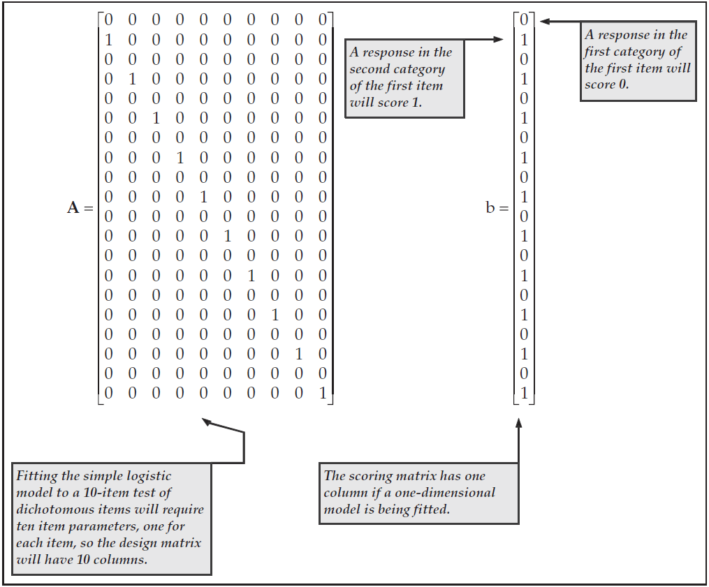
Figure 3.1: Design and Scoring Matrices for a Simple Logistic Model Fitted to Data Collected with 10 Dichotomous Items

For polytomous data, a model such as Masters’ partial credit model (Masters, 1982) can be used. Suppose, for example, that we wish to fit a partial credit model to three items, each with four response categories. This can be achieved with the design and score matrices shown in Figure 3.2.

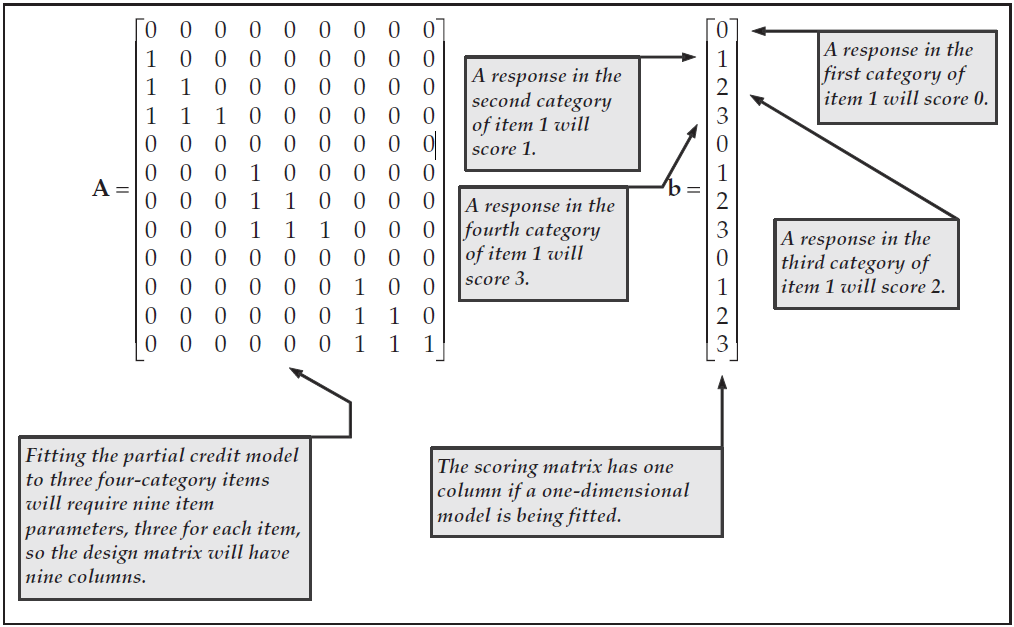
Figure 3.2: Design and Scoring Matrices for a Partial Credit Model Fitted to Data Collected with Three Polytomous Items

The models in both Figure 3.1 and Figure 3.2 are unidimensional, that is, they assume that all of the items are indicators for a single latent variable. Both can easily be altered to become multidimensional models through the respecification of the scoring matrices. In Figure 3.3, we show two scoring matrices that, if used as alternatives to the scoring matrices in Figures 3.1 and 3.2, would result in two- and three-dimensional models respectively.

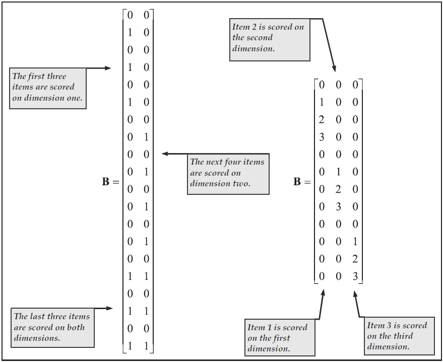
Figure 3.3: Multidimensional Scoring Matrices for Dichotomous and Polytomous Data

As a final example, Figure 3.4 shows the design and scoring matrices that can be used for multifaceted data. Consider an example of a rating context in which students’ work is rated against two criteria by two raters and that each rating uses a three-point scale, scored 0, 1, 2. To fit the generalised Rasch model to such data, the combination of the two criteria and the two raters are regarded as four generalised items. Assuming the generalised items are defined in the sequence criterion 1, rater 1; criterion 1, rater 2; criterion 2, rater 1; criterion 2, rater 2; then the matrices in Figure 3.4 fit a two-faceted Rasch model that posits a unique rating structure for each generalised item.

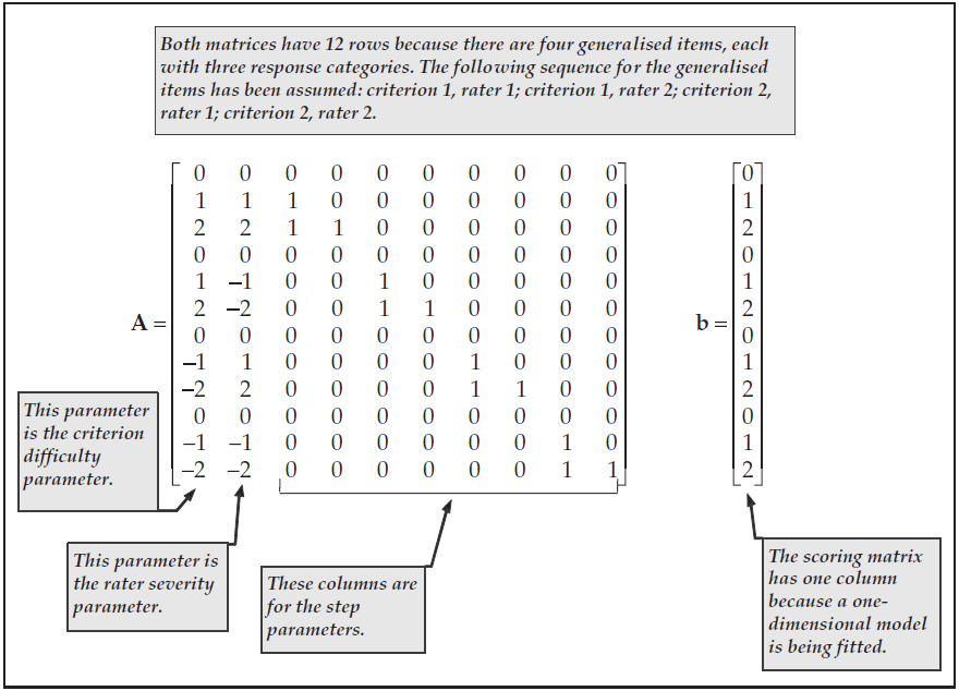
Figure 3.4: Design and Score Matrices for a Multifaceted Polytomous Model

The form of the parameterisation that has been used in Figure 3.4 follows that of Andrich (1978). Ten parameters are used. The first column provides a criterion difficulty parameter, the second provides a rater severity parameter, and columns three to ten are the step parameters.

Even though the data are collected using two criteria, the item response model includes a single criterion difficulty parameter: the design matrix has set the difficulty of the second criterion to be the negative of the difficulty of the first criterion.

This kind of constraint is often applied to identify the item response model and is equivalent to setting the mean of the criteria parameters to zero.⁴³ Similarly, the model in Figure 3.4 uses a single rater severity parameter, with the severity of the second rater set to be the negative of the severity of the first rater.⁴⁴

The structure of these design and score matrices can, perhaps, be best understood by noting from (3.5) that

\[\begin{equation} \log \left(\frac{\operatorname{Pr}\left(X_{i j}=1 ; A, B, \xi | \theta\right)}{\operatorname{Pr}\left(X_{i j-1}=1 ; A, B, \xi | \theta\right)}\right)=\left(b_{i j}-b_{i j-1}\right) \theta+\left(a_{i j}^{\prime}-a_{i j-1}^{\prime}\right) \xi \text{.} \tag{3.50} \end{equation}\]

3.1.6.2 The Structure of ACER ConQuest Design Matrices

ACER ConQuest can import user-defined design matrices, or it can generate its own design matrices by drawing upon the command code that is used to specify a model. Section 2.10, Importing Design Matrices provides two sample analyses that use user-defined design matrices. For many models, however, ACER ConQuest command code can be used so that appropriate design matrices are automatically generated.

The score matrix cannot be imported, but the ACER ConQuest score command can be used to generate score matrices. The relationship between the score command and the score matrix is direct and need not be described here.

The design matrix is generated from the ACER ConQuest model statement, the syntax of which is described in the command reference ( Chapter 4, ACER ConQuest Command Reference). The full details of how the design matrix is generated are beyond the scope of this manual; however, it is useful to note how the basic structure of the design matrix is determined.

In the model statement, four types of terms can used: terms that involve a single variable, terms that involve the product of two or more variables, the term step, and terms that involve the product of step and other variables.

ACER ConQuest must first determine the number of rows in the score and design matrices. It does so by noting all of the different variables used in the model statement and then examining the data to identify all possible combinations of the levels of the variables. Each possible combination is called a generalised item. Each valid response category for a generalised item constitutes one row in the score matrix and one row in the design matrix. The valid response categories are all categories between the lowest and highest category found in the data for the generalised item.⁴⁵

A set of parameters (columns of the design matrix) is then generated for each term in the model. If the term involves a single variable, then the number of parameters generated is one less than the number of levels in that variable.⁴⁶ If the term involves the product of two or more variables, then the number of parameters generated is \((K_1 - 1)(K_2 - 1)(K_3 - 1)...\), where \(K_i\) is the number of levels in the \(i\)-th variable used in the term. If the term is step, then the number of parameters generated is two less than the maximum of the number of categories in all of the generalised items. If the term involves step and other variables, the number of parameters generated is \(\sum_t (L_t - 2)\), where the summation is over all of the combinations of levels of the variables that are in the term (of course, excluding step) and \(L_t\) is the maximum of the number of categories in those generalised items that include the \(t\)-th combination of variables.

ACER ConQuest then proceeds to construct a design matrix that is based upon the Andrich (1978) parameterisation of polytomous Rasch models. If an imported matrix is used as a replacement for the generated matrix, then each row of the imported matrix must refer to the same category and generalised item as those to which the corresponding row of the generated matrix refers. No constraint is placed on the number of columns (parameters) in the imported matrix.

3.1.7 Traditional Item Statistics

The itanal command displays a variety of traditional item statistics, most of which are self-explanatory. To assist in their discussion, however, it is important to define the ACER ConQuest concept of raw score. The raw score for a case is the sum of the scores achieved by a case divided by the maximum possible score that the case could have achieved. More formally, if we let \(\Xi_n\) be the set of generalised items to which case \(n\) responded, then the raw score \(s_n\) for case \(n\) is defined as

\[\begin{equation} s_{n}=\frac{\sum_{i \in \Xi} b_{i x_{n i}}^{*}}{\sum_{i \in \Xi} b_{i K_{i}}^{*}} \text{,} \tag{3.51} \end{equation}\]

where \(b_{i x_{n i}}^{*}\) is the sum across the dimensions of the score that has been assigned to category \(x_{ni}\) of item \(i\).

3.1.7.1 Discrimination

The discrimination index that is printed for each item (see, for example, Figure 2.31) is the product moment correlation between the case scores on this item, \(b_{i x_{n i}}^{*}\), and the corresponding case raw scores, \(s_n\). Only those cases who responded to the item are included in the calculation.

3.1.7.2 Point Biserial

For each response category of an item, a point-biserial correlation and \(t\)-statistic are computed. To compute the point biserial for category \(k\) on item \(i\), a dummy variable \(y_{ikn}\) is constructed so that

\[\begin{equation} y_{ikn}=\left\{\begin{array}{cc} 1 & \mbox{if case n has responded in category k of item i}\\0 & \mbox{otherwise}\end{array}\right. \text{.} \tag{3.52} \end{equation}\]

The point biserial is then the correlation between the set of values \(y_{ikn}\) and the corresponding case raw scores \(s_n\). Only those cases who responded to the item are included in the calculation.

If the data set is complete and the items are dichotomously scored, then the discrimination index and the point biserial for the category that is scored 1 will be equal. If the data set is incomplete, this does not hold.

The \(t\)-statistic provides a significance test for the point biserial. The degrees of freedom for the statistic are two less than the total number of students who responded to the item. Since this will normally be greater than 30, the t-statistic can be treated as a normal deviate.

3.1.7.3 Summary Statistics

The mean, variance, skewness and kurtosis statistics (see, for example, Figure 2.13) that are reported at the end of an itanal run are scaled to a metric that assumes that every case responded once to every item. The Cronbach’s alpha coefficient of reliability (which is equal to KR-20 when all items are dichotomously scored) and the standard error of measurement also assume that every case responded once to every item. Further, they are not reported if more than 10% of the response data is missing (compare, for example, Figure 2.13 with Figure 2.32).

---

37. The current version of ACER ConQuest does not compute standard errors for the multidimensional form of the model.↩︎

38. The current version of ACER ConQuest uses the Monte Carlo method only when producing EAP ability estimates and variances for those ability estimates.↩︎

39. The value of this constant can be set with the set command argument zero/perfect=r.↩︎

40. The value \(M\) should be large. The default value in ACER ConQuest is \(2000\). The value of the ACER ConQuest set command argument p_nodes=n controls the value of \(M\).↩︎

41. In ACER ConQuest, the number of nodes used to approximate the integrals in (3.48) and (3.49) is governed by the set command argument f_nodes=n, and the number of random draws used by the Monte Carlo integration method is governed by fitdraws=n. The default value of f_nodes is \(2000\), and the default value of fitdraws is \(1\).↩︎

42. Note, however, that a model using the matrices in Figure 3.1 will only be identified if the mean of the latent variable, \(\mu\), is constrained to be zero.↩︎

43. As an alternative to setting the mean of a set of parameters to zero, it may be possible to identify the model by setting the mean of the latent variable to zero. This is what would have been required to identify the models in Figures 3.1 and 3.2.↩︎

44. In the multifaceted case, setting the mean of the latent variable to zero removes the requirement of setting the mean of one set of parameters to zero only.↩︎

45. The lowest and highest categories are determined as follows. ACER ConQuest identifies all valid codes (after recoding) and then sorts those codes (using an alphanumeric sort) to find the lowest and highest category.↩︎

46. When the set command argument lconstraints=cases is used and the term is the first term, the number of parameters generated is equal to the number of categories of the variable in the term.↩︎